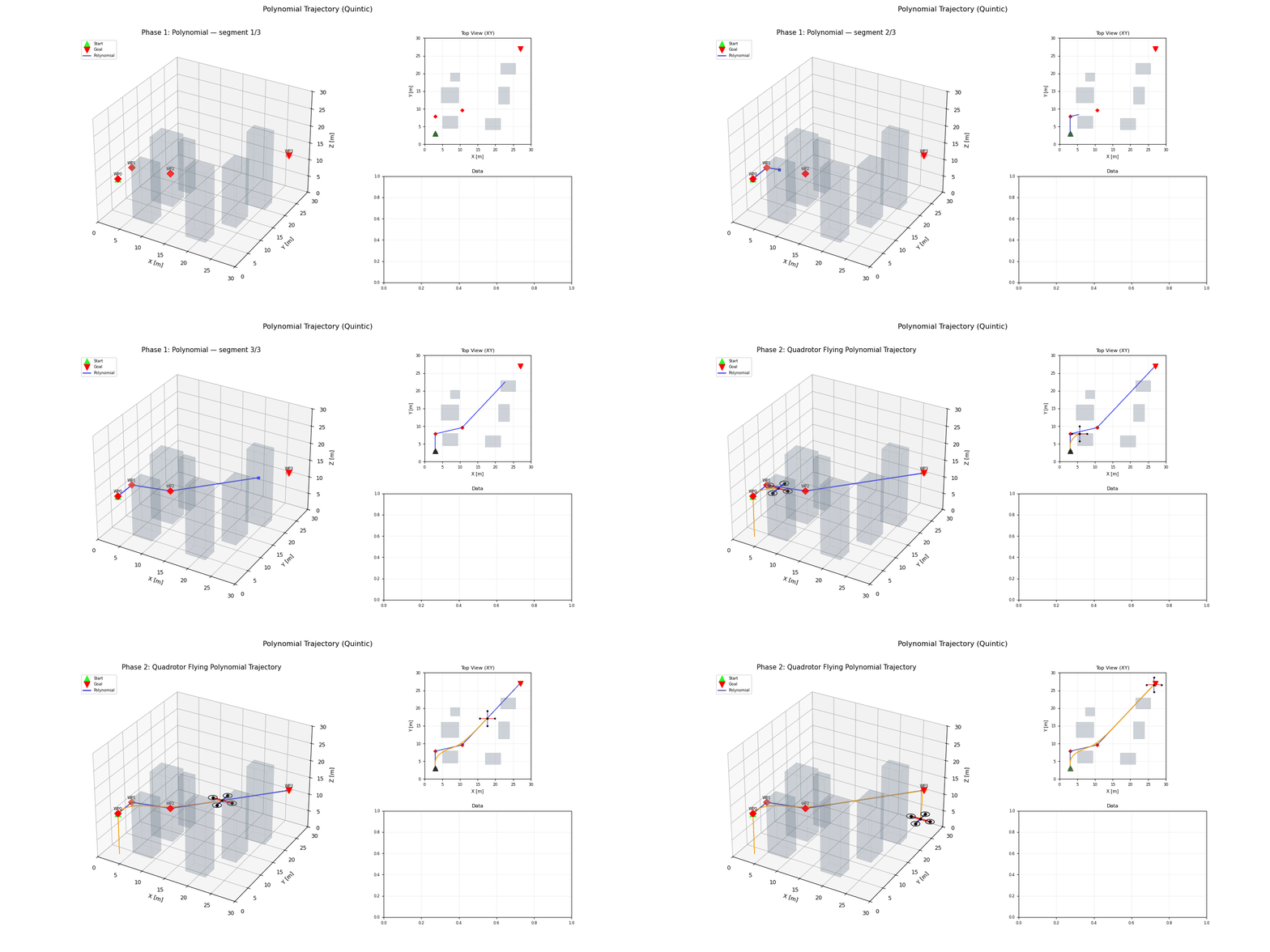
Polynomial Trajectory

Problem Statement

Piecewise polynomial trajectories provide a flexible middle ground between simple waypoint interpolation and full optimal control. They are useful when smoothness requirements are moderate and realtime generation is required.

Model and Formulation

For segment j, define polynomial p_j(t) and enforce continuity at knot k:

$$p_j(t_k)=p_{j+1}(t_k),{\dot{p}}_j(t_k)={\dot{p}}_{j+1}(t_k),{\ddot{p}}_j(t_k)={\ddot{p}}_{j+1}(t_k)$$

The system reduces to linear equations over coefficient vectors.

Algorithm Procedure

1. Define knot times and boundary conditions.
2. Assemble linear system for polynomial coefficients.
3. Solve for each axis independently (or jointly with coupling constraints).
4. Sample trajectory for planner/controller interfaces.

Tuning Guidance

• Ensure knot timing matches available acceleration authority.
• Prefer lower polynomial degree for numerical stability.
• Add regularization if coefficient solving is ill-conditioned.

Failure Modes and Diagnostics

• Poorly spaced knots produce high curvature and controller stress.
• Under-constrained systems cause non-unique solutions.
• High polynomial degree can cause oscillatory artifacts (Runge-type behavior).

Implementation and Execution

python -m flybots.simulations.trajectory_planning.polynomial_trajectory

Evidence

References

• Siciliano et al., Robotics: Modelling, Planning and Control
• LaValle, Planning Algorithms

Related Algorithms

• Quintic Polynomial
• Minimum Snap