MPC Path Tracking

Problem Statement

Linear MPC uses the same hover-linearised model as LQR, but re-solves a finite-horizon optimal control problem every step and applies only the first input. That buys two things LQR cannot offer: explicit input constraints, and preview of where the reference is going.

Model and Formulation

At each control step:

min_{u_{0 : N - 1}} \sum_{k = 0}^{N - 1} (‖ x_{k} - x_{k}^{r e f} ‖_{Q}^{2} + ‖ u_{k} ‖_{R}^{2}) + ‖ x_{N} - x_{N}^{r e f} ‖_{Q_{f}}^{2}

subject to x_{k+1} = A_d x_k + B_d u_k and u_min ≤ u_k ≤ u_max.

Preview Is the Whole Point

Note the x_k^{ref} — indexed by k, one reference per horizon step. Holding a single reference point across the horizon asks the plan to come to rest where the trajectory happens to be right now, and reduces MPC to an LQR with a slower solver and a worse constant lag. Sampling the reference forward is what makes it a different controller:

python

preview = [reference(t + k * ctrl_dt) for k in range(horizon + 1)]
wrench = mpc.compute(
    state,
    np.array([p[0] for p in preview]),
    target_vel=np.array([p[1] for p in preview]),
)

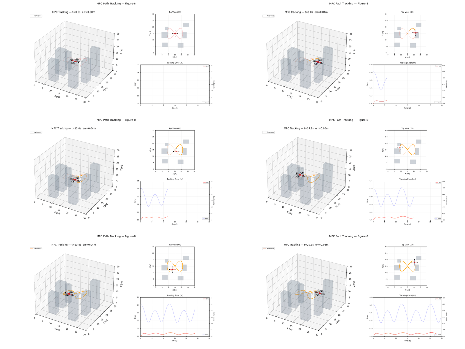
On the atlas figure-8: 0.395 m mean error held, 0.032 m with preview.

The Terminal Cost Has to Match the Discretisation

Q_f approximates the cost-to-go beyond the horizon, and it must come from the discrete algebraic Riccati equation when the running cost is summed per step rather than integrated. A continuous-time solution under-weights the terminal state by a factor of 1/dt — at dt = 0.05 that is 20× — and the horizon effectively ends in mid-air.

Algorithm Procedure

Discretise the hover linearisation once, offline; solve the discrete ARE for Q_f.
Sample the reference across the horizon.
Warm-start from the previous solution, shifted by one step.
Solve the bounded QP, apply u_0, discard the rest.

Tuning Guidance

Longer horizons buy more preview and cost solve time. What matters is how far ahead the horizon reaches in seconds, not how many knots it has — lengthen the step before adding knots.
Input bounds are where MPC earns its keep over LQR; set them from the actual actuator, not as slack.
Warm-starting is not optional at these rates: from cold, the solver spends its iteration budget re-finding the previous answer.

Failure Modes and Diagnostics

A constant lag proportional to reference speed means the preview is not wired up.
Too few solver iterations shows up as jitter, not as an error message.
Bounds tight enough to make the problem infeasible produce whatever the solver returns on failure.

Implementation and Execution

bash

python -m uav_sim.simulations.path_tracking.mpc_tracking

Evidence

MPC Tracking

MPC Path Tracking ​

Problem Statement ​

Model and Formulation ​

Preview Is the Whole Point ​

The Terminal Cost Has to Match the Discretisation ​

Algorithm Procedure ​

Tuning Guidance ​

Failure Modes and Diagnostics ​

Implementation and Execution ​

Evidence ​

References ​

Related Algorithms ​